Cube AI – Remixed

Cube AI is an experimental AI project. The objective was to create a neural network that can solve a Rubiks Cube. This project started life as a command line application, that modelled the Rubiks cube and attempted to solve the puzzle using a single layer neural network.
I’ve revisited this project to change it to use a more sophisticated multi layer perceptron neural network and added a web user interface to demonstrate the AI in action.
To achieve this goal the I had to overcome the following challenges:
- Modelling a cube
- Implementing a multi layer perceptron neural network
- Implementing a 3D vector graphics presentation layer
- Training the neural network to learn how to solve a muddled cube
- Testing the neural network against an unseen muddled cube
Cube AI performs well in testing. With 82 hidden nodes the AI is able to solve most cubes with up to 19 moves. Testing indicates that this could be improved by more training and adding more nodes to the hidden layers.
Cube AI is implemented in Typescript with a React UI, backed by Redux toolkit and 99% test coverage.
Cube AI is available at cube-ai.cmatts.co.uk.
Modelling
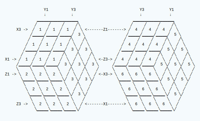
The Cube object models a Cube with Faces. Faces have rows and columns that map to the face colour matrix. The cube has 6 faces and can perform 6 actions.
- Rotate plane 1 (X1) – F
- Rotate plane 2 (X3) – B
- Rotate plane 3 (Y1) – L
- Rotate plane 4 (Y3) – R
- Rotate plane 5 (Z1) – U
- Rotate plane 6 (Z3) – D
Through these simplified actions all moves can be achieved.
Cube Axis
Rotate actions apply to each face as follows:

Each face is mapped internally as a matrix represented rows and columns of colour numbers. Rows for each face are mapped from top to bottom on the above diagram and columns are mapped from the left to right. This is for ease of visualisation.
Neural Network
This solution uses a Multi Layer Perceptron feedforward neural network to map input tuples to a set of output nodes. There is one output node for each possible action.
Multi Layer Perceptron

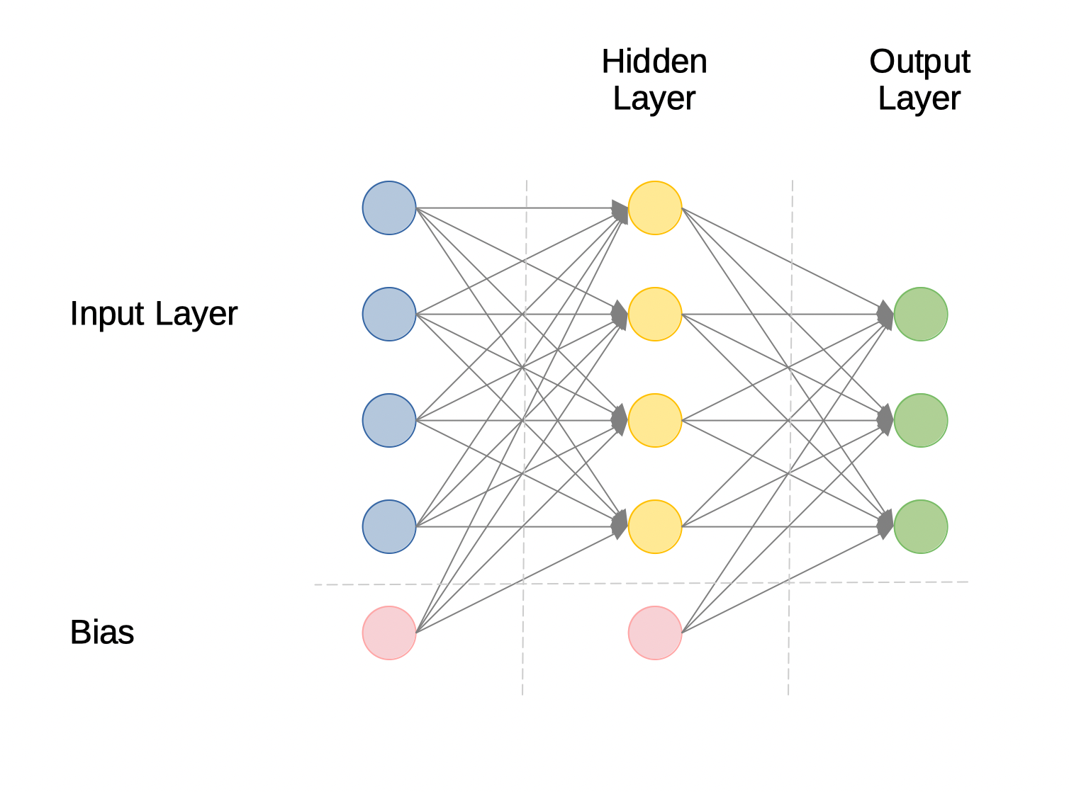
A Multi Layer Perceptron is a fully connected neural network that comprises an input layer, one or more hidden layers and an output layer.
The input layer is a set of nodes that represent the input from the problem domain. Each node is connected to all the nodes in the adjacent hidden layer. Similarly, all the nodes in that hidden layer are connected to all the nodes in its adjacent hidden layer or the output layer in there are no more hidden layers.
In addition, each layer has a bias node that is connected to all the nodes in that layer.
The connections between nodes have a weight associated with them.
When an input set is presented to any layer, the input is multiplied by the connection weight to calculate the input to be applied to each connected node. Each node calculates the sum of its inputs and applies a sigmoid function to determine the output of that node, which in turn becomes the input to the next layer. This process is called feedforward and is repeated for all nodes in all layers until we have a set of output values. The winning output is the node with the greatest sum of all its inputs.
Bias nodes are not connected to inputs and always have an input value of 1. Using the bias as a weighted input serves to create a distinction on the between the outputs for each node.
The sigmoid function serves to convert the linear input to a sigmoid curve output where only a strong input will result in a strong output. This enables the network to learn complex non-linear problems.
\(\delta\left( x \right) = \biggl[ \frac{1}{1 + \left(e^{-x}\right)} \biggr]\)
The derivative sigmoid function is used to calculate the gradient of the
Training
When training the network, data is presented as a set of tuples. Where a tuple is a collection of values representing the input source. Each value in the tuple is mapped to a specific input node.
The network calculates the output for each node and feeds that forward through each layer until a winning output node is determined.
The actual output is subtracted from expected output for each output node to calculate the error. This error is then used to calculate a gradient to be applied to each of the input weights that feed that node.
The gradient is the error multiplied by the derivative input multiplied by a learning rate.
Each weight is multiplied by its error gradient to calculate a weight delta. The weigh delta is then added to the weight to apply an adjustment. When all the input weights for the layer have been adjusted, the error for the preceding layer is calculated by multiplying the output weights by the previous error. The layer error is then used to feedback and adjust the input weights on that layer and so the process repeats until the weights from the input layer have been adjusted.
If the outcome was correct then the weighting is increased to re-enforce the selection, otherwise the weighting is decreased to discourage the selection.
Node weights are initialised using a pattern similar to Xavier weight initialisation, where the weights are uniformly distributed and bound by the following equation:
Where
Network Configuration
To work with this particular problem, the network is configured with 288 input nodes that correspond to the cube state. It has one hidden layer comprising 82 nodes, and 6 output nodes corresponding to the possible actions.
The number of hidden layers and nodes in each layer has been selected through extensive experimentation.
Initial tests showed that the optimal number of nodes for learning quickly is 82 with 1 hidden layer. Increasing the number of hidden layers slowed down learning significantly.
User Interface
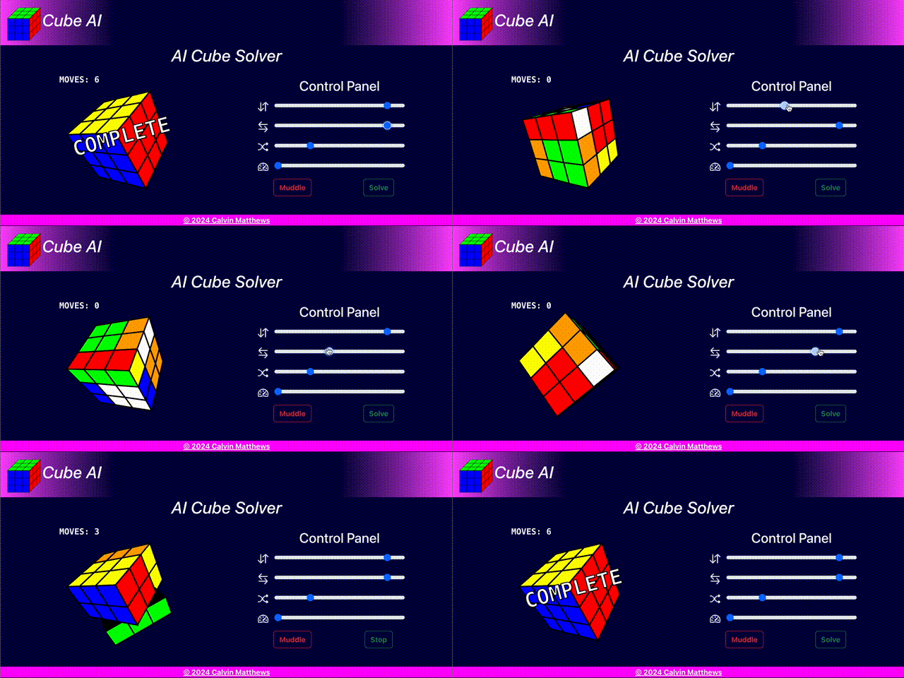
Cube AI provides a web based user interface from which to demonstrate and test the neural network.
The user interface comprised a cube view and a control panel. It is implemented using React backed by Redux Toolkit state management.

Cube AI is available at cube-ai.cmatts.co.uk.
Cube View
The cube view presents a 3D view of the Rubiks cube. The view is generated using SVG.
Each block in the cube is modelled as an object in 3 dimensional space with 6 sides. The cube comprises 27 such blocks. The sides of the blocks are represented as tiles in that 3 dimensional space. Inner tiles are allocated a colour of black and outer tiles are allocated the colour of the corresponding face colour for the Cube State. Blocks are subjected to the following transformations:
- X plane rotation
- Y plane rotation
- Z plane rotation
- X cube rotation
- Y cube rotation
- Z cube rotation
- Scale multiplier
- Perspective multiplier
The X, Y and Z plane rotations are used to rotate the blocks for a face when animating moves. The X, Y, and Z cube rotations enable the cube to be rotated to view all sides.
The scale multiplier is used to scale the model for presentation and the perspective multiplier applies distance perspective for 2D viewing.
The resulting output is a set of 2D tile vectors that are sorted by distance and layered on top of each other to produce a 3 dimensional impression of the cube.
Control Panel
The control panel enables:
- Changing the difficulty level
- Creating a new muddled cube
- Starting the AI solver
- Changing the speed of the AI solver
- Rotating the cube view
Solving the Cube
Learning Moves
In order to solve the cube the system needs to learn to recognise what moves are appropriate for the state of a muddled cube. This is achieved by muddling a new cube and training the neural network to select the appropriate action to reverse the move made at each stage. The system will then attempt to solve the muddled cube to evaluate training progress.
Note: Training moves are in reverse so that the network can be trained to select the forward move to get back to the previous state.
Training is performed based on a difficulty setting that determines how many moves to learn against a new cube. This process is repeated for n number of training cycles, each time using a different random seed to ensure that the moves are varied and that solution moves are re-enforced.
The bigger the training difficulty the greater the number of possible states, and the more training cycles are required.
Through experimentation, I found that the network scales best when trained on the greater difficulties first and then retrains on the lower difficulties. Training on the greater difficulties tends to unlearn earlier training. Taking this approach, the lower difficulties nearest the complete state become re-enforced, whilst there is some knowledge of the cube state at greater difficulties retained.
Cube State
The state of the cube is presented to the neural network as a tuple constructed from the faces of the cube.
Each face piece is represented by an array of 6 binary digits, where one of the 6 is set to 1 to represent the colour and the others are 0. This is done for every face piece except the centre pieces. Centre pieces never change, so they are not mapped. All of these binary representations are combined to form one large tuple consisting of 288 input values (6 * 6 * 8).
Solve
The system is presented with an unseen muddled cube and attempts to solve the puzzle. This process requires presenting the cube state to the neural net and applying the triggered action and is repeated until the cube is either complete, a maximum number of moves have been applied or a stuck state is detected.
Results
After extensive training with a mixed set of difficulty the network is able to complete simple puzzles and some more complex puzzles.
The above chart shows the performance of the network, when presented with 1000 puzzles at each difficulty level.